Six AI Inference Chips: The Cheapest Wasn't Fastest

TL;DR: The lowest-priced accelerator is not always the cheapest way to serve tokens. Fit the weights and KV cache in memory, compare bandwidth per dollar, then measure delivered-token cost at your latency target. The result is a decision matrix, not a universal chip winner.

Key Takeaways: - Memory capacity is a gate. Memory bandwidth per dollar shapes decode economics. - TTFT, ITL, per-user throughput, and aggregate throughput must agree with the cost result. - Compare platforms at equal quality, concurrency, and service levels.

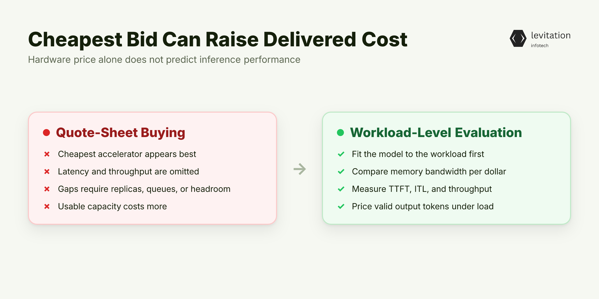
Our six-path comparison found that the lowest-priced accelerator did not produce the fastest result. The paradox disappears once quote-sheet price is separated from serving performance. LLM production depends on time to first token, inter-token latency, throughput under load, and inference cost per token.

A purchase price is not a service-level agreement. A cheap accelerator that misses TTFT or ITL can force extra replicas, queues, or headroom. Those changes turn a low quote into a higher delivered-token cost.

That is the false economy: paying less for hardware while paying more for usable capacity.

The six paths examined were: - NVIDIA H200 - AMD MI300X - Groq LPU - Google TPU v5e/v6 - AWS Trainium - Intel Gaudi 3

The TPU and Trainium entries represent platform paths, not individual SKUs. Each path also includes instance shape, networking, orchestration, compilers, and runtime versions.

Track the operating result, not the catalogue number: - Time to first token and inter-token latency - Per-user and aggregate throughput - Cost per million valid output tokens at the required latency - Accelerator-memory capacity - Memory bandwidth per dollar

The qualitative result was clear. Lower acquisition cost did not guarantee faster performance. Groq's low-latency design did not always outperform mature NVIDIA H100/H200 deployments.

That does not make Groq slow. It makes hardware type a weak proxy for workload performance.

Training and inference optimize different goals. AI/ML training rewards throughput across optimization steps. Inference must meet latency and unit economics for every generated token.

The reusable rule is simple: fit the model first, compare bandwidth per dollar next, then calculate delivered-token cost under your own workload. That rule leads to the divergence inside the decode loop, where the accelerator waits for data instead of doing arithmetic. What exactly is it waiting for?

Decode waits for data. During autoregressive generation, each new token requires the model to read weights and the request's KV cache.

Peak FLOPs describe arithmetic capacity. They do not measure how quickly the accelerator can fetch state for each decode step. The fetch path behind Inside the AI Brain explains why that distinction matters.

Start with a hard gate: Do the model weights fit in accelerator memory?

Then budget for the KV cache. Context length, request concurrency, and the serving runtime determine how much additional memory each request consumes.

Model fit alone is not enough. A model can fit with room to spare, then exhaust that memory when several long conversations arrive together.

For NVIDIA systems, start with a simple inventory command:

Use each vendor's equivalent inventory tool for TPU, Trainium, and Gaudi deployments. Can that memory feed each decode step quickly enough?

Decode repeatedly reads model weights and KV-cache state. Memory bandwidth therefore offers a more useful early signal than peak FLOPs or isolated TOPS.

Bandwidth per dollar gives a practical first ranking. It estimates decode work supported per dollar before serving software and workload shape enter the result.

It is a screening metric, not a universal law. A well-tuned runtime can shift a chip's practical position. How does the chip behave when requests arrive together?

Batching can improve aggregate utilization by sharing device work across requests. Under heavier batching, queueing or per-user latency can rise. Throughput and latency must be read together.

Groq makes the trap visible. Very low latency does not guarantee faster performance than a mature H100/H200 configuration on every workload.

An AI/ML training result cannot settle this question. It measures a different phase with a different bottleneck.

Use this diagnostic sequence:

1. Confirm model fit.
2. Reserve memory for KV cache and concurrency.
3. Compare memory bandwidth per dollar.
4. Test concurrency behavior.
5. Measure serving-software efficiency.

That order prevents a generic GPU-versus-ASIC debate from hiding the real constraint. Once the bottleneck is visible, the six paths split into three performance modes. Which mode fits the workload best?

The comparison produced classes of fit, not a single podium.

NVIDIA H200 is the general-purpose default in this set. Its upgraded memory and bandwidth matter, as does its mature serving-software ecosystem.

Choose it when model fit, latency, portability, and operational maturity all matter. What changes when capacity becomes the binding constraint?

AMD MI300X is a capacity-first alternative for large FP16 models where lower VRAM cost matters. That is workload fit, not a claim that MI300X wins every inference test.

Its case strengthens when capacity is the binding constraint and the serving stack supports your model cleanly. Which options target latency or service cost instead?

Groq, Google TPU, AWS Trainium, and Intel Gaudi 3 belong in focused comparisons. Each should be tested against a defined latency or cost target.

Read the results as a decision matrix, with no unsupported overall rank: - H200: Broad model fit, mature software, and a strong general-purpose production profile. - MI300X: Capacity-first fit for large FP16 models where lower VRAM cost matters. - Groq: Latency-first candidate that still needs workload-level throughput and cost testing. - TPU v5e/v6: Platform path worth testing for stable workloads and integrated cloud operations. - Trainium: AWS platform path worth testing when portability and cloud integration fit. - Gaudi 3: Alternative path that must justify itself through delivered-token cost and stack compatibility.

Compare every option on fit, bandwidth per dollar, latency, delivered-token cost, software maturity, and workload stability. How much of the chip's ceiling can the software unlock?

Chip selection sets the ceiling. Serving software determines how much of that ceiling production reaches.

That software includes: - Compiler quality - Attention and paging kernels - Quantization support - Orchestration - Model compatibility - Operational tooling

Groq is the central counterexample to purchase-price thinking. Specialized hardware can be very fast, but not uniformly faster than an expensive, mature GPU platform.

But those performance classes still have to be measured on the same workload before a procurement decision can survive scrutiny. How can the benchmark make that comparison credible?

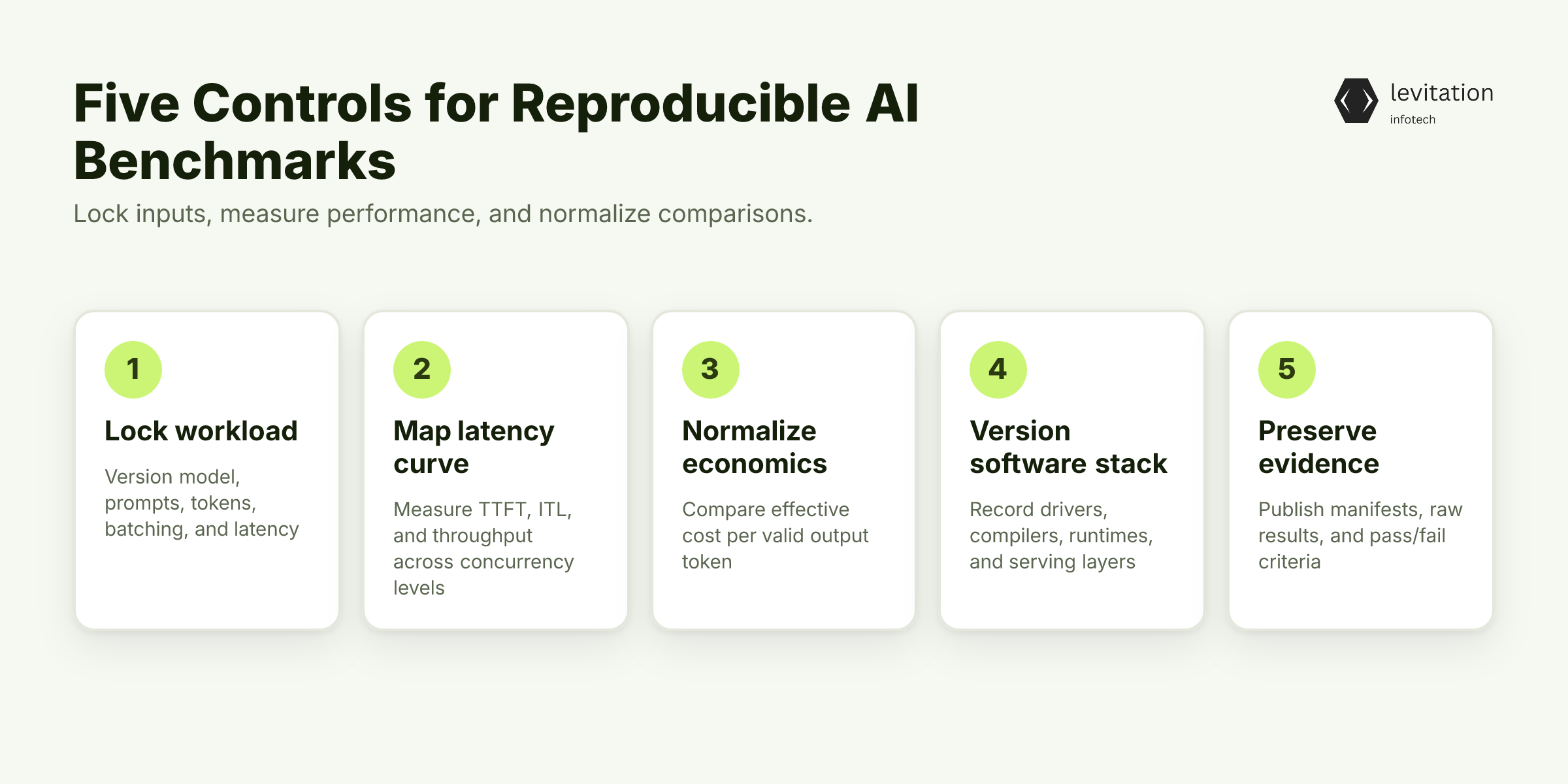
A decision matrix is only as credible as the workload behind it. Otherwise, it is six marketing claims arranged in attractive columns.

Fix the model revision, weights, precision, quantization, prompts, input and output lengths, context, batching, concurrency, and latency target.

Start with a machine-readable manifest:

Null fields should block the run. Changing one hidden input can reverse the result. Which latency point still qualifies as production-ready?

Test each platform across several concurrency levels. Measure TTFT, ITL, per-user throughput, aggregate throughput, and output tokens per hour.

Report two operating points: the fastest observed result and the best point that still satisfies the service-level objective.

A fastest point that misses the SLO is not a production result. What does that production-ready point cost?

Calculate effective inference cost per token:

“Valid” means completed at the required latency and quality bar.

Use the same accounting boundary for every platform. Do not compare a raw chip price with a vendor's cloud-service quote.

Compare memory bandwidth per dollar under the same workload. Otherwise, the economic comparison inherits different software and utilization assumptions. Which stack produced those tokens?

Record the accelerator count, driver, compiler, runtime, serving framework, attention kernel, quantization method, and orchestration layer. Without those fields, another team cannot reproduce the result.

Cross-check findings with several complementary tools: - InferenceMAX provides living, multi-vendor benchmark data. - InferenceBench publishes modeled and signed benchmark records. - SageMaker AI's AIPerf workflow measures endpoint latency and throughput.

External reference, not a comparison row: Treat vendor-reported figures, including NVIDIA's inference performance reference, as external context. Compare them only after verifying that the workload, serving stack, and measurement method match.

Keep that reference outside the six-path matrix. A different workload and serving stack make direct comparison misleading.

Publish the configuration, prompt hash, raw measurements, and pass/fail criteria. A leaderboard image cannot replace reproducibility.

With comparable numbers in hand, the benchmark becomes a constraint-first buying guide. Which constraint should come first in your deployment?

Comparable numbers still do not choose hardware by themselves. A model that misses memory cannot be rescued by low latency. A platform that misses the SLO cannot be rescued by low cost.

Start with the mature GPU path for changing models, short-lived workloads, or teams without accelerator-specific optimization skills. Treat specialized silicon as a targeted exception. How should that burden shape the comparison?

Compare each option on: - Model fit - TTFT and ITL - Cost at the target service level - Software maturity - Workload portability - Operational burden

The accounting formula needs measured inputs, not catalogue estimates:

For custom ASICs, demand a stable workload profile and high utilization before accepting migration risk. Low silicon cost cannot repair poor model fit, software friction, or idle capacity.

Traffic shape can overturn an average. Your AI Cost Dashboard Lies About Bursts shows why burst behavior belongs in the comparison.

Run a short pilot with production-shaped prompts, representative context lengths, realistic concurrency, and the intended serving stack. Re-run it when the model, software, or traffic changes.

The practical payoff is not a universal chip winner. It is a decision that reaches production faster without buying the wrong bottleneck. Which procurement changes follow?

Procurement changes in three concrete ways: - Price screens become delivered-token cost comparisons. - Latency specialists become workload-specific options. - Accelerator selection starts with memory fit, not headline compute.

Turn the scorecard into a living decision artifact. Model formats, serving kernels, and accelerator software evolve quickly.

Update the comparison whenever the model, runtime, compiler, orchestration layer, traffic pattern, or service target changes. Stop Bleeding Money on LLM Inference explains why serving architecture matters beyond the accelerator.

Keep AI/ML training evidence in a separate lane. It answers a different operating question and cannot validate serving economics.

That operating judgment should be grounded in production, not only laboratory data.

The best accelerator meets the workload's latency target at the lowest delivered-token cost. It must also use an operating model the team can sustain. Which procurement questions should come first?

Which AI inference chip is fastest for LLMs?

There is no universal fastest chip. Groq delivers very low latency, but it does not always match NVIDIA H100/H200 deployments. H200 is a common production default because its serving ecosystem is mature.

The answer changes with model fit, concurrency, traffic shape, and the latency target. A benchmark from AI/ML training cannot settle it.

What is the most important metric for AI inference TCO?

Inference cost per token at a defined service-level target is the most complete economic metric. Pair it with TTFT, ITL, and throughput.

A cheap platform that misses the required latency is not cheaper in production. Re-run the calculation when quality or traffic changes.

Are custom ASICs always cheaper than GPUs?

No. Dedicated inference chips win for specific cost-or-latency profiles with stable workloads. Software maturity, model compatibility, utilization, and migration cost can outweigh lower silicon cost.