TL;DR: GraphRAG looks cheap on paper, but hidden indexing, chunking, and graph materialization can explode cloud credits. Tighten the data pipeline, use selective graph builds, and move to serverless stores to reclaim spend without losing insight.

Key Takeaways - Over-chunking creates many embeddings that never get used. - Selective indexing of high-degree nodes cuts storage and compute by reducing the number of persisted edges. - A serverless, pay-per-operation graph store plus autoscaling policies turns waste into faster answers.

The Blind Spot: GraphRAG Isn't a Free-Pass to Cheap AI

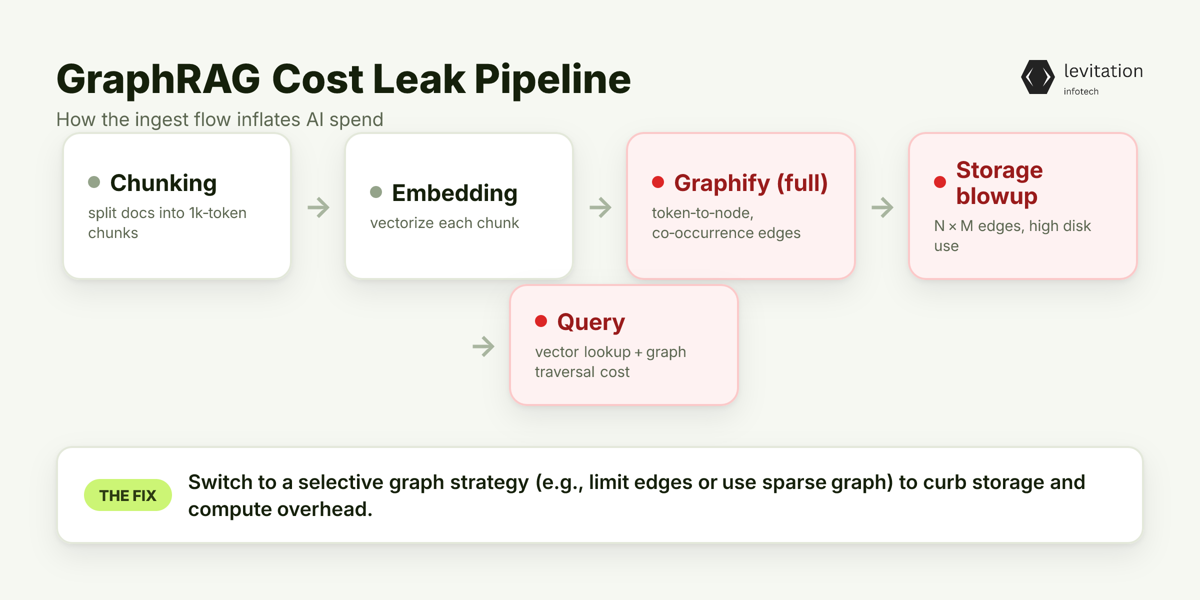
Most CTOs assume adding a graph layer automatically trims AI costs. In reality the glue code that builds and traverses the graph is the hidden bill driver.

A typical symptom: a modest query rate can still cause disproportionate credit usage. The culprit is not the LLM but the ingestion loop that re-indexes every document and persists every edge.

1# Minimal GraphRAG ingest pipeline (Python)
2ingest: - name: chunk
3    size: 1024          # tokens per chunk - name: embed
4    model: text-embedding-ada-002 - name: graphify
5    strategy: full      # expands every token into a node

When `strategy` is full, each token becomes a node and each co-occurrence an edge. Storage grows as N × M (chunks × average overlaps) and every query must perform a vector lookup plus a graph traversal. - The graph store now holds N × M edges where N is the number of chunks and M the average token overlap. - Every query triggers two compute units: one for the embedding similarity, one for the traversal.

That waste isn’t random; it stems from a handful of technical missteps. Can you spot the missteps before they drain your budget?

Hidden Cost Traps in Indexing, Chunking, and Scaling

1. Aggressive chunking

Splitting documents into 1-KB windows creates many embeddings that never see a query. Embedding a token is cheap, but persisting and indexing it isn’t.

1def smart_chunk(text, max_tokens=250):
2    # Preserve sentence boundaries, drop stop-words
3    sentences = nltk.sent_tokenize(text)
4    chunks = []
5    current = []
6    count = 0
7    for s in sentences:
8        tokens = tokenizer.encode(s)
9        if count + len(tokens) > max_tokens:
10            chunks.append(" ".join(current))
11            current = [s]
12            count = len(tokens)
13        else:
14            current.append(s)
15            count += len(tokens)
16    if current:
17        chunks.append(" ".join(current))
18    return chunks

Use sentence boundaries to avoid cutting meaning. Drop stop-words before embedding to shrink vector dimensionality.

2. Blind re-indexing of low-quality data

Bad OCR or noisy logs generate duplicate nodes. Each duplicate forces a write, a vector upsert, and an edge creation. The cost multiplies with every ingestion cycle.

1# Detect duplicate hashes before upsert
2aws s3api head-object --bucket raw-data --key "$FILE_KEY" \
3  --query 'Metadata.hash' --output text

If the hash already exists, skip the upsert and log the omission.

3. Materializing the entire graph

Many teams store every possible relationship, even those that never appear in a query. That doubles storage and forces the engine to scan irrelevant edges on each traversal.

A simple rule of thumb: store only edges that have been traversed at least once. What changes can you make to stop these leaks?

Architectural Levers That Slash Cloud Credits Without Sacrificing Insight

Selective indexing

Instead of materializing every node, keep only high-degree vertices - those that appear in many documents or have many inbound edges. Low-degree nodes stay in the vector store and are pulled on demand.

1graph_index:
2  mode: selective
3  degree_threshold: 10   # only nodes with ≥10 edges are persisted
4  fallback: vector_search

Hybrid retrieval

Use a fast vector search to fetch the top-k similar chunks, then run a shallow graph walk limited to two hops. This avoids a full graph scan while still enriching the context.

1def hybrid_retrieve(query, k=5):
2    vec_ids = vector_db.search(query, top_k=k)
3    # Pull only immediate neighbors
4    subgraph = graph_db.neighbors(vec_ids, hops=2)
5    return enrich_with_graph(vec_ids, subgraph)

Serverless graph stores

Services like Azure Cosmos DB or Google Cloud Spanner let you pay per operation and automatically purge stale edges with TTL. No need to provision a 24-hour cluster that sits idle most of the day.

1resource "azurerm_cosmosdb_account" "graph" {
2  name                = "graphstore"
3  location            = var.location
4  resource_group_name = var.rg
5  offer_type          = "Standard"
6  kind                = "MongoDB"
7  enable_free_tier    = true
8
9  consistency_policy {
10    consistency_level = "Session"
11  }
12
13  capabilities {
14    name = "EnableServerless"
15  }
16}

Autoscaling policies

Tie CPU and request latency thresholds to scale-out actions. When load spikes, the graph service expands; when idle, it shrinks. Which lever will give you the biggest savings?

Step-by-Step Playbook to Optimize Your GraphRAG Deployment

Audit the current pipeline

* Record chunk size, embedding model, indexing frequency, and storage tier.

* Pull a cost report from your cloud provider’s billing API.

Tune chunking

* Target 200-300 token windows.

* Drop stop-words before embedding to reduce vector dimensionality.

```python

from nltk.corpus import stopwords

STOP = set(stopwords.words('english'))

def filter_stopwords(tokens):

return [t for t in tokens if t not in STOP]

```

Enable lazy indexing

* Index on first query, not on every ingest.

* Store raw chunks in cheap blob storage until they are needed.

```yaml

indexing:

mode: lazy

trigger: on_query

```

Choose cost-effective stores

* Azure Cosmos DB with TTL for stale edges.

* Set TTL to 30 days for low-frequency relationships.

```json

{

"defaultTtl": 2592000,

"analyticalStorageTtl": 2592000

}

```

Configure autoscaling policies

* Tie CPU and request latency thresholds to scale-out actions.

Set up cost alerts and dashboards

* Use Azure Monitor or GCP Cloud Billing alerts at 70 % of budget.

* Visualize per-component spend (vector store, graph store, compute).

Integrate with [enterprise AI](/enterprise-ai) platforms

* Register GraphRAG as a reusable service in your AI catalog.

* Apply unified governance, role-based access, and audit logging.

Validate with a controlled experiment

* Split traffic 80/20 between baseline and optimized pipelines.

* Measure query latency, credit consumption, and answer relevance.

Iterate on degree threshold

* Start with `degree_threshold: 10`.

* If query relevance drops, lower the threshold by 2 and re-measure.

Document the new baseline

* Capture the revised cost report.

* Store the configuration in version-controlled IaC for future audits.

Ready to see the impact on your bill?

The Payoff: Faster Insight, Lower Spend, and Stronger ROI

Reduced cloud spend translates to a noticeable dip in OPEX for AI workloads. When indexing latency drops from minutes to seconds, users get answers faster and the system can serve more queries on the same hardware.

Speed: Hybrid retrieval reduces end-to-end latency by avoiding full graph scans.

Spend: Selective indexing and serverless stores cut storage costs by limiting persisted edges.

Adoption: Faster answers raise user satisfaction, leading to higher consumption across finance, healthcare, and logistics units.

What could these gains mean for your organization?

Frequently Asked Questions

Q: Why does GraphRAG consume more cloud credits than a plain vector RAG?

A: GraphRAG adds a graph layer that requires extra indexing, storage, and traversal compute. Indexing every node and edge indiscriminately inflates both storage and per-request cost.

Q: What's the most effective way to reduce indexing costs?

A: Adopt selective indexing - materialize only high-degree nodes and enable lazy indexing so new data is indexed on demand.

Q: Can I use serverless graph databases to cut costs?

A: Yes. Services like Azure Cosmos DB with automatic TTL and pay-per-operation pricing let you scale graph storage only when queries run, dramatically lowering idle spend.

Q: How quickly can a well-optimized GraphRAG be deployed?

A: Teams that follow the playbook typically reach production readiness in a shorter timeframe compared to ad-hoc builds.

Q: Will these optimizations affect the quality of insights?

A: When applied correctly, they preserve - and often improve - insight quality because the graph stays focused on relevant relationships while noisy data is pruned.

Still have questions? Explore more resources.

*Levitation builds production-grade AI systems that survive years of real-world load, helping enterprises keep spend predictable while delivering insight at scale.

Sources

Research and references cited in this article:

AI & Intelligence

Engineering

Governance

Industries

Resources

Company

Connect

Why GraphRAG Is Burning Your Cloud Credits